Getting Started
What you need
Our framework is built around AWS cloud services. Make sure that:
- You have access to an AWS account.
- You have installed the AWS command line interface (CLI) on your machine:
$ pip3 install awscli --upgrade --user - You have configured AWS CLI with your AWS access key ID and secret:
$ aws configure AWS Access Key ID [None]: AKIAIOSFODNN7EXAMPLE AWS Secret Access Key [None]: wJalrXUtnFEMI/K7MDENG/bPxRfiCYEXAMPLEKEY Default region name [None]: us-east-1 Default output format [None]: json - You have created an Amazon machine image (AMI) for each of the nodes (satellites, base stations) in your constellation. For simplicity, you can create a single AMI with all the necessary software and start different programs on each node.
Installing VCE
You can install VCE on your local machine as follows:
$ git clone https://github.com/isi-rcg/vce
$ cd vce
$ make init
VCE requires Python 3.7 and InfluxDB 1.7.6.
Configuring a Constellation
The simplest example is one with just a satellite and a base station.
Configuration is done using a single YAML file, which will be called
config.yml in this example:
system:
  awscli: 'aws'                          # local command for AWS cli
  stackname: vce                         # AWS cloudformation stack name, instance tags
  zone: us-east-1a                       # AWS zone where instances are started
  keyname: paolieri                      # SSH key associated with instances
  server:                                # configuration for the VCE server
    hostname: vce                        #   hostname
    type: c4.4xlarge                     #   VM type
    ami: ami-0bd0790a4f69961da           #   VM image
    snap: snap-000e53be3d99a21c1         #   data partition snapshot
    user: centos                         #   VM username
  db:                                    # configuration of timeseries db (InfluxDB)
    name: vce
    host: vce
    port: 8086
  orbits:
    start: 2019-02-15 13:50:00           # UTC, start time of orbits simulation
    step: 1.0                            # in minutes, frequency of orbits recalculation
    duration: 30.0                       # in minutes (orbit simulation stopped afterward)
  agent_interval: 0.5                    # in seconds, frequency of VM agent polling VCE server
  metrics_interval: 2.0                  # in seconds, frequency of collected metrics
  start_delay: 2                         # as integer minutes, delay before running instance cmd

satellites:
  - hostname: iss
    type: c4.4xlarge
    ami: ami-0bd0790a4f69961da
    snap: snap-000e53be3d99a21c1
    user: centos
    cmd: |
      echo Running ping sequence...
      fping -l -p 15000 -D arlington
    tle1: '1 25544U 98067A   19040.02956382  .00000286  00000-0  11897-4 0  9995'
    tle2: '2 25544  51.6414 278.5526 0005375   9.1011 131.7761 15.53240808155340'

stations:
  - hostname: arlington
    type: c4.4xlarge
    ami: ami-0bd0790a4f69961da
    snap: snap-000e53be3d99a21c1
    user: centos
    cmd: ''
    lat: 38.882737
    lon: -77.105993
    alt: 78.0
Three VMs will be started: one for the satellite node iss, one for
the ground station arlington, and one for the VCE server vce. For
simplicity, we are using the same VM type (c4.4xlarge) and AMI
(ami-0bd0790a4f69961da) for all nodes.
The framework will automate several tasks:
- It will install VCE on all VMs.
- It will install a time series database (InfluxDB 1.7.6) and
metrics visualization webserver (Grafana 6.2.0) on the VM that
is used for the VCE server (
vce). - It will install and configure a collector of system statistics (collectd 5.8.1) on each ground station or satellite VM.
- It will configure
/etc/hostson each VM, assigning the host namesvce,iss,arlingtonto the IP addresses of the VMs on their private network (e.g.,10.0.1.1,10.0.1.2,10.0.1.3). This simplifies the configuration of programs running in the constellation: you can just runping arlingtonfromiss. - It will start the VCE server on
vceand the VCE agent onissandarlington: the agent will query the current bandwidth/delay of each link from the server and apply them to its VM using the Linux NetEm module. - Finally, it will run the given command
cmdon each instance. In this example, the satellite nodeisswill send ping probes to the ground stationarlingtonevery 15 seconds.
Analyzing Satellite Orbits
In our example, we used a two-line element set (TLE) from CelesTrak NORAD for the international space station (ISS) and the latitude and longitude coordinates of Arlington, VA.
Before starting a simulation on AWS, it is useful to check the orbits
that will be used by the VCE server to emulate network parameters.
You can check satellite orbits locally on your machine (the following
commands assumes that vce is available on the system PATH;
alternatively, you can type alias vce='pipenv run python -m vce' and
run them from its installation directory):
$ export HOSTALIASES=hosts
$ vce db reset config.yml
Deleting database vce...
Creating database vce...
$ vce orbits compute config.yml
Setting HOSTALIASES allows using localhost as an alias of vce
for local testing. The first command vce db reset config.yml resets
the time series database; vce orbits compute config.yml computes the
position of each satellite every minute (step: 1.0) for the next 30
minutes (duration: 30.0) from the initial time (start: 2019-02-15
13:50:00).
You can visualize them on a 2D map:
$ vce orbits plot2d config.yml example.pdf

For each point on the orbit, a line connecting the satellite to the base station is drawn if there is line of sight. VCE ensures that VMs of base stations and satellites can exchange messages only when there is line-of-sight, with latency computed from their distance.
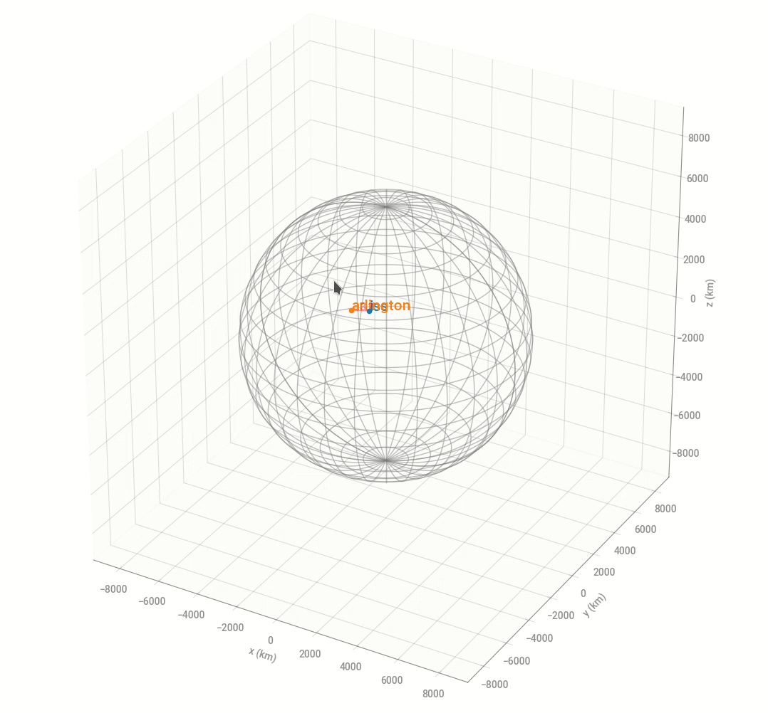
Orbits can also be visualized in 3D and explored interactively:
$ vce orbits animate config.yml --interactive orbits.gif
Running on AWS
VCE leverages AWS CloudFormation to make it easy to configure, start and stop several VM instances. You can generate a YML CloudFormation template using VCE:
$ vce cloud stack demo/config.yml > stack.yml
This command will create the file stack.yml with all of the
necessary instructions to start a stack of virtual machines on AWS,
one for each satellite or base station (with the VCE agent
preinstalled) and one for the VCE server.
To actually create your stack on AWS, you can run:
$ aws cloudformation create-stack --stack-name vce --template-body file://./stack.yml
{
    "StackId": "arn:aws:cloudformation:us-east-1:300950145788:stack/vce/5b378a00-813f-11e9-9b5a-0e94a1882570"
}
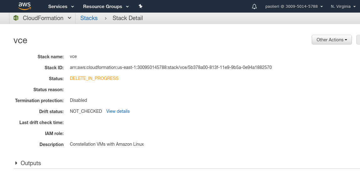
You check the state of the stack creation in the AWS console of your account, inside “CloudFormation”:

After a couple of minutes (or more, depending on the number of started
VMs), the status of the stack should turn into “CREATE_COMPLETE”. By
clicking on “vce” (the name of the stack), you can check the allocated resources:

Clicking on the “Physical ID” of a resource such as the IssInstance,
you can check its properties, including the public and private IP
addresses.
You can use these to enter the node and manually check its logs:
$ ssh -i ~/.ssh/paolieri.pem centos@18.234.220.16
[centos@iss ~]$ cat cmd.out
Running ping sequence...
[1559044680.784812] arlington : [0], 84 bytes, 0.22 ms (0.22 avg, 0% loss)
...
Note how, in the VCE configuration config.yml, the cmd parameter
of node iss was
    cmd: |
      echo Running ping sequence...
      fping -l -p 15000 -D arlington
These commands are run in the home directory /home/centos and the
output (stdout and stderr) is saved into cmd.out:
[centos@iss ~]$ cat cmd.out
Running ping sequence...
[1559646120.949065] arlington : [0], 84 bytes, 0.34 ms (0.34 avg, 0% loss)
[1559646135.956754] arlington : [1], 84 bytes, 6.81 ms (3.57 avg, 0% loss)
[1559646150.957949] arlington : [2], 84 bytes, 6.76 ms (4.63 avg, 0% loss)
[1559646165.959216] arlington : [3], 84 bytes, 6.79 ms (5.17 avg, 0% loss)
[1559646180.960440] arlington : [4], 84 bytes, 6.79 ms (5.49 avg, 0% loss)
[1559646195.963848] arlington : [5], 84 bytes, 8.99 ms (6.08 avg, 0% loss)
[1559646210.965060] arlington : [6], 84 bytes, 8.98 ms (6.49 avg, 0% loss)
[1559646225.966297] arlington : [7], 84 bytes, 9.01 ms (6.80 avg, 0% loss)
[1559646240.967510] arlington : [8], 84 bytes, 9.01 ms (7.05 avg, 0% loss)
[1559646255.971169] arlington : [9], 84 bytes, 11.4 ms (7.49 avg, 0% loss)
[1559646270.972317] arlington : [10], 84 bytes, 11.4 ms (7.85 avg, 0% loss)
[1559646285.973526] arlington : [11], 84 bytes, 11.4 ms (8.15 avg, 0% loss)
[1559646300.974737] arlington : [12], 84 bytes, 11.5 ms (8.41 avg, 0% loss)
[1559646315.978508] arlington : [13], 84 bytes, 14.1 ms (8.81 avg, 0% loss)
[1559646330.979631] arlington : [14], 84 bytes, 14.1 ms (9.17 avg, 0% loss)
[1559646345.980756] arlington : [15], 84 bytes, 14.0 ms (9.47 avg, 0% loss)
[1559646360.981888] arlington : [16], 84 bytes, 14.0 ms (9.74 avg, 0% loss)
Note how the RTT changes from 0.3 to 6.8 ms right after the start of
the simulation, increasing over time as iss moves away from arlington.
You can also access (in real time) the entire time series database of
measurements (CPU, memory, disk, interfaces) collected from the
different nodes (satellites and base stations) by the VCE server. To
do this, you need to create an SSH tunnel from your computer to the
VceInstance; using the AWS web console, find the IP address of this
node (54.242.51.197 in this example), then run:
$ ssh -i ~/.ssh/paolieri.pem -NL 3000:localhost:3000 centos@54.242.51.197
You can now access Grafana (running on the VCE server in AWS) from your computer by opening http://localhost:3000.
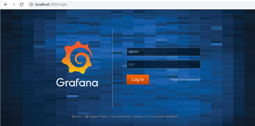
The initial username and password are both admin.
To visualize the metrics from the time series database:
- Click on
Add data source>InfluxDB - Type
http://localhost:8086as URL andvceas database name.
You can create custom dashboards with metrics from the database.
You can deallocate all AWS resources with:
$ aws cloudformation delete-stack --stack-name vce